Types of Data in Statistics & Data Science

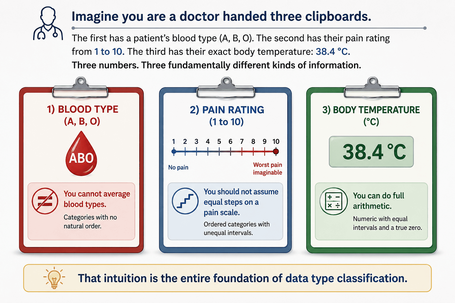
What Are Types of Data in Statistics?

In statistics and data science, a data type describes the nature of values within a variable — what those values mean, what operations are mathematically valid on them, and consequently which analytical methods are appropriate. Getting this wrong is not a minor academic concern. It determines which statistical test you run, which machine learning algorithm you use, which visualization the data faithfully versus misrepresents it, and which database storage format you choose.

Core Definition

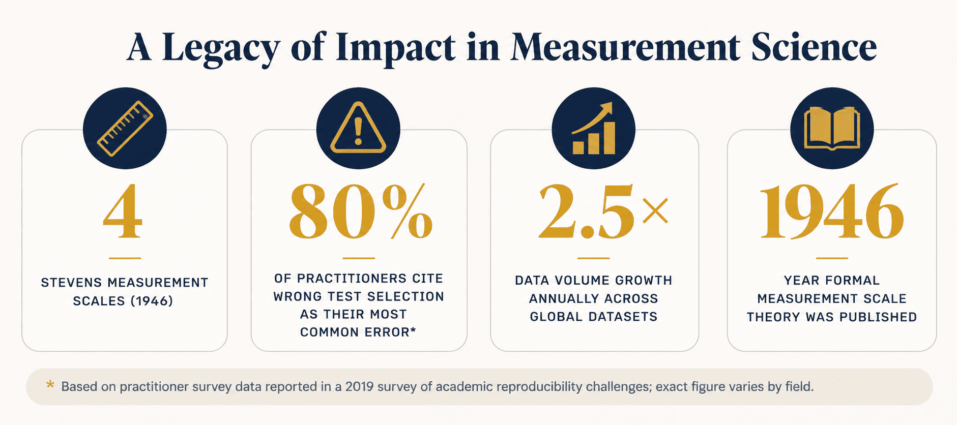
Data type (also called measurement level or scale of measurement) serves as a classification system which defines all mathematical characteristics of a variable — including its allowed operations, applicable comparison methods, and valid statistical summaries. The dominant framework which psychologist S.S. Stevens proposed in 1946, defines four levels which are: nominal, ordinal, interval, and ratio.

Why is classification important beyond academic formality? There are four practical reasons for this:

• Statistical test validity — applying a t-test to nominal categories produces meaningless results.

• ML algorithm selection — tree-based models handle nominal data natively; linear regression does not.

• Visualization fidelity — a histogram is meaningful for continuous data; a pie chart suits nominal.

• Storage efficiency — encoding gender as a two-bit categorical is far cheaper than a full float.

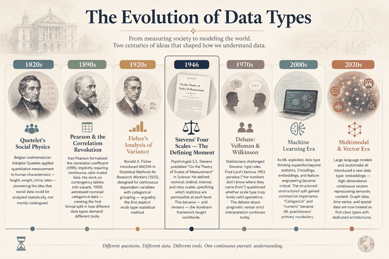
History & Origin of Data Classification

Classification of measurement did not spring into being fully formed. It evolved across two centuries of scientific practice, philosophical debate, and computational necessity.

 

 

"The statistics of a given body of data depend on the measurement scale employed, and the selection of an appropriate statistic requires that the investigator know or assume the scale of measurement represented in his data."

— S.S. Stevens, "On The Theory of Scales Of Measurement," Science, Vol.103, No.2684 (1946)

Read Also: Data Science & Big Data Project Ideas and Topics for Final Year CS Students

The Master Classification Map

Data types in statistics and data science form a rich hierarchy. The top-level split is between Qualitative (categorical, descriptive) and Quantitative (numerical, measurable) data. Within these, further distinctions apply based on scale properties.

 

 

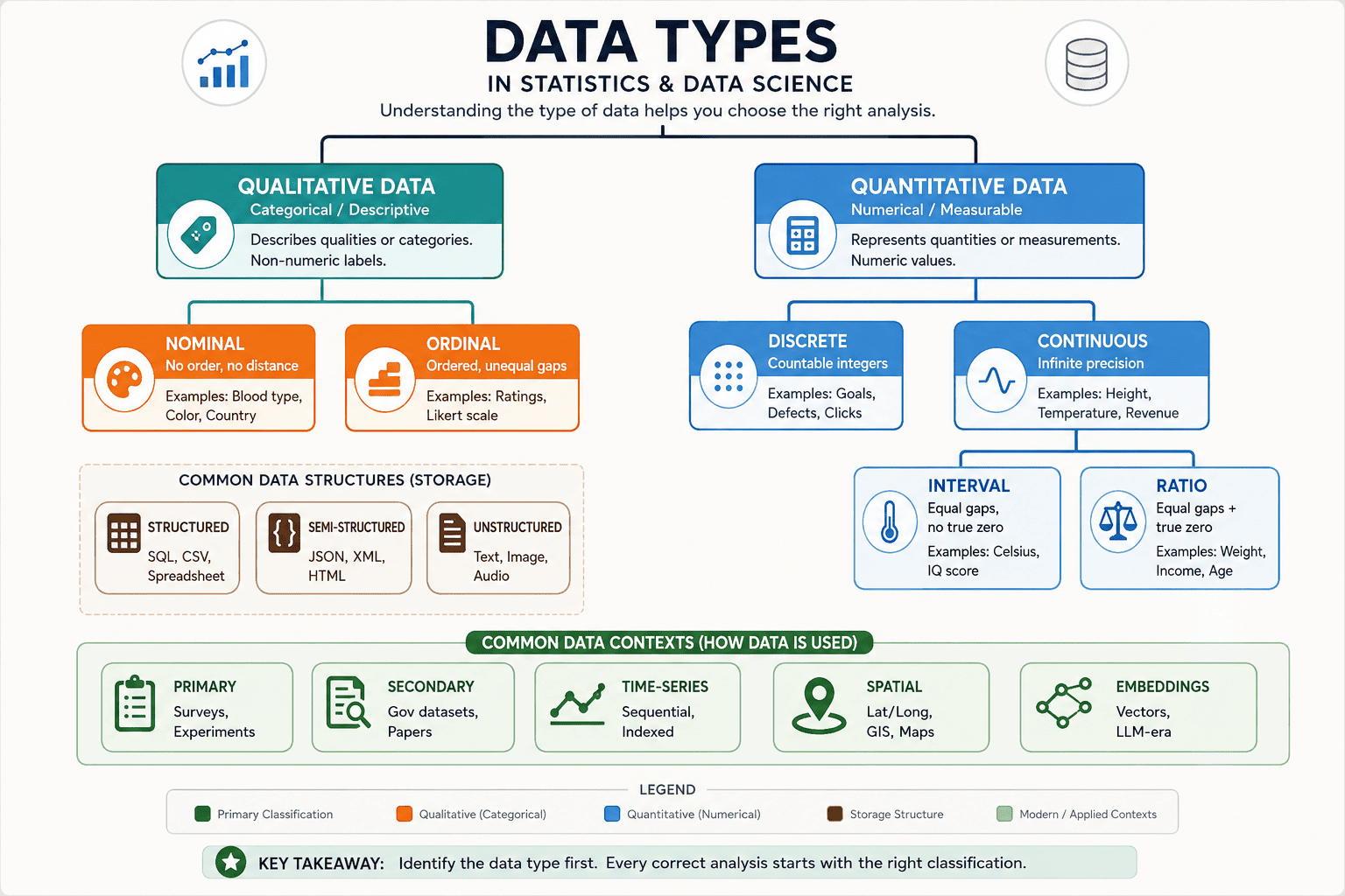
The classical Stevens hierarchy (nominal → ordinal → interval → ratio) has additive properties — each level includes all capabilities of the level below it, plus one more. Ratio data can do everything interval data can, plus form meaningful ratios. Ordinal can do everything nominal can, plus rank. This structure directly governs which mathematical operations are valid.

"Data quality is not just about accuracy or completeness. A perfect accurate blood-type label, if treated as an interval number in a regression, produces nonsense. The type of the variable is itself a form of metadata — and ignoring it is one of the most common analytical errors in applied research."

— Velleman, P.F. & Wilkinson, L., "Nominal, Ordinal, Interval, And Ratio Typologies Are Misleading," The American Statistician, 47(1), 1993

Nominal Data — Deep Dive

Nominal data is the most fundamental category. Values are labels — names for distinct groups with no inherent order and no numeric meaning. The word "nominal" comes from the Latin nomen (name). 

Characteristics & Examples

Blood type (A, B, AB, O), country of birth, product category, browser type, eye color, gender identity, car brand — these are classic examples of types of data examples in the nominal class. No category is "greater than" another. You can ask whether values are equal or different, nothing more.

What You Can Do

• Mode — the most frequent category is meaningful.
• Frequency counts & percentages — how many items fall into each class.
• Chi-square test — test association between two nominal variables.
• Visualize with bar charts, pie charts, treemaps.

What You Cannot Do

• Mean or median — "average blood type" is meaningless.
• Ranking — there is no intrinsic order.
• Arithmetic operations — subtracting "red" from "blue" has no interpretation.
• Pearson correlation — assumes numeric distance, invalid here.

Encoding Nominal Data for Machine Learning

# Encoding Nominal Data — One-Hot, Label, and Target Encoding

import pandas as pd

import numpy as np

from sklearn.preprocessing import OneHotEncoder, LabelEncoder

from category_encoders import TargetEncoder

df = pd.DataFrame({

    'blood_type': ['A', 'B', 'O', 'AB', 'A', 'O'],

    'country':    ['IN', 'US', 'DE', 'IN', 'BR', 'US'],

    'target':     [1, 0, 1, 1, 0, 1]

})

# 1. ONE-HOT ENCODING  — best for low-cardinality nominal features

ohe = OneHotEncoder(sparse_output=False, handle_unknown='ignore')

ohe_result = ohe.fit_transform(df[['blood_type']])

ohe_df = pd.DataFrame(ohe_result, columns=ohe.get_feature_names_out())

print(ohe_df)

# 2. LABEL ENCODING — integer codes; only safe for tree-based models

le = LabelEncoder()

df['blood_type_label'] = le.fit_transform(df['blood_type'])

print(df[['blood_type', 'blood_type_label']])

# ⚠️  Label encoding implies order — risky for linear models!

# 3. TARGET ENCODING — replaces category with mean of target

#    Ideal for high-cardinality features (e.g., zip codes, countries)

te = TargetEncoder()

df['country_target'] = te.fit_transform(df['country'], df['target'])

print(df[['country', 'country_target']])

Common Mistakes

• Label encoding for linear models — label-encoding "dog=0, cat=1, fish=2" tells a linear model fish is twice cat. Use one-hot instead.

• High-cardinality one-hot — one-hot encoding a column with 500 unique countries creates 500 binary columns, causing dimensionality explosion. Use target or frequency encoding.

• Treating nominal as numeric — storing zip codes as integers and computing their mean is a classic error in data pipelines.

 

Ordinal Data — Deep Dive

Ordinal data adds one property that nominal lacks: meaningful order. The categories have a natural ranking, but the gaps between ranks are not necessarily equal. [Qualitative]

Characteristics & Examples

Education level (high school < bachelor's < master's < doctorate), customer satisfaction (dissatisfied → neutral → satisfied → very satisfied), military rank, pain scale (1–10), star ratings — these are prototypical ordinal examples. We know "satisfied" is better than "neutral," but we cannot say it is exactly twice as good.

What You Can Do

• Median & mode — valid central tendency measures.
• Percentile & quartiles — rank-based summaries.
• Spearman rank correlation — measures monotonic association between ordinal variables.
• Mann-Whitney U, Kruskal-Wallis — non-parametric tests comparing groups.

What You Cannot (Strictly) Do

• Arithmetic mean — averaging "strongly agree (5)" and "strongly disagree (1)" to get "neutral (3)" assumes equal intervals — an assumption the data does not support.
• Pearson correlation — requires equal intervals.
• Standard deviation — distance-based; meaningless without equal gaps.

Nominal vs Ordinal — Comparison Grid

Nominal Data	Ordinal Data
Categories have no intrinsic order	Categories have a meaningful order/rank
Any permutation of labels is equally valid	Order is fixed and meaningful
Mode is the only valid central tendency	Median and mode valid; mean debated
Chi-square test for association	Spearman r, Kruskal-Wallis for tests
One-hot encoding standard for ML	Ordinal encoding preserves rank
Examples: blood type, country, product color	Examples: satisfaction rating, education level

The Likert Scale Controversy: Ordinal or Interval?

The question "is Likert scale data ordinal or interval?" is one of the longest-running debates in applied statistics. A standard Likert item asks respondents to rate agreement on a 5- or 7-point scale (1 = Strongly Disagree … 5 = Strongly Agree). Strictly, this is ordinal — we cannot prove the psychological distance from 2 to 3 equals the distance from 4 to 5.

Yet decades of empirical research (notably Norman, 2010) show that when scales have 5+ points and distributions are approximately symmetric, treating them as interval and computing means yields results consistent with more rigorous non-parametric approaches. Many social science and healthcare journals therefore accept mean scores from Likert scales as conventional practice. The practical decision requires you to understand the assumption which you should present with full transparency and choose non-parametric tests for situations when distribution shows skewness or your sample size remains limited.

# Encoding Ordinal Data — Preserving Order

import pandas as pd

from sklearn.preprocessing import OrdinalEncoder

df = pd.DataFrame({

    'education': ['High School', 'Bachelor', 'Master', 'PhD', 'Bachelor'],

    'satisfaction': ['Low', 'High', 'Medium', 'Very High', 'Low']

})

# Define the explicit order (critical — don't let sklearn guess!)

edu_order = [['High School', 'Bachelor', 'Master', 'PhD']]

sat_order = [['Low', 'Medium', 'High', 'Very High']]

enc_edu = OrdinalEncoder(categories=edu_order)

enc_sat = OrdinalEncoder(categories=sat_order)

df['education_enc'] = enc_edu.fit_transform(df[['education']])

df['satisfaction_enc'] = enc_sat.fit_transform(df[['satisfaction']])

print(df)

# Output: education_enc — 0,1,2,3 correctly ordered

# satisfaction_enc — 0,2,1,3 — respects Low

# Spearman correlation between ordinal variables

from scipy.stats import spearmanr

corr, p = spearmanr(df['education_enc'], df['satisfaction_enc'])

print(f"Spearman r = {corr:.3f}, p = {p:.3f}")

Discrete Data — Deep Dive

Discrete data is quantitative and countable — values are whole numbers (integers) with no possible values between them. You can have 3 children or 4, but not 3.7. [Quantitative]

Characteristics and Examples 

Number of goals scored in a match, page views per day, defects per manufactured unit, number of customer complaints per week, number of students in a class, book counts — these exemplify discrete data. The set of values is countable, even if theoretically infinite (e.g., page views per day could be any non-negative integer).

Statistical Tools for Discrete Data

• Poisson distribution — models count events occurring at a constant rate in a fixed interval (calls per hour, typos per page).
• Negative Binomial — handles overdispersed count data (variance > mean), common in healthcare and ecology.
• Count regression (Poisson GLM) — models a count outcome as a function of predictors.
• Bar charts with integer bins — correct visualization; do not use continuous histograms.

Discrete vs Continuous Intuition

If you can ask "how many?" → discrete. If you can ask "how much?" → continuous. "How many people?" is discrete. "How much time?" is continuous.

Continuous Data — Deep Dive

Continuous data can take any value within a range — including infinitely many values between any two observations. Height of 172.354 cm is valid. Revenue of $1,847.33 is valid. No "gaps" exist in the value space. [Quantitative]

Interval vs Ratio Distinction

This is the subtlest and most misunderstood split in Stevens' hierarchy. Both interval and ratio data are continuous with equal spacing between values. The difference is a true zero.

Interval Scale	Ratio Scale	Practical Implication
Equal gaps, no meaningful zero. Example: Temperature in Celsius. 0 °C does not mean "no temperature" — it is an arbitrary reference point. IQ scores, calendar dates. You can add/subtract (20 °C warmer), but ratios are meaningless (40 °C is not "twice as hot" as 20 °C in any physical sense).	Equal gaps plus a meaningful zero. Zero means "none of the attribute." Weight, height, income, reaction time, age. All arithmetic is valid. 80 kg is genuinely twice 40 kg. This is the richest data type and permits the widest range of statistical analysis.	Most ML algorithms treat interval and ratio identically. The distinction matters primarily when interpreting ratios in scientific conclusions. "Country A's GDP is 3× Country B's" requires ratio scale. "City A is 10° warmer than City B" requires only interval.

What Type of Data Is Age?

Age is a classic interview question. Age is ratio data — it has a true zero (birth), equal intervals (each year is one year), and meaningful ratios (40 years old is twice 20 years old). However, when age is reported in bins ("18–24," "25–34"), it becomes ordinal — the binning destroys continuous precision. Always note whether you have raw age (ratio) or age group (ordinal).

Statistical Tools for Continuous Data

• Mean, standard deviation — valid measures of center and spread.
• Normal distribution, t-distributions — model continuous variation.
• t-tests, ANOVA — compare continuous means across groups.
• Pearson correlation, linear regression — model linear relationships.
• Histograms, KDE plots, box plots — reveal distributional shape.

Structured vs Unstructured vs Semi–Structured Data

Alongside the classical measurement hierarchy, a parallel classification describes the form of data storage. This is the dominant framing in data engineering and commercial data science.

Structured Data 

Organized into rows and columns with a predefined schema. Every cell has a known data type, every column a name. SQL databases, spreadsheets, CSV files, and most data warehouses hold structured data. Tools like SQL, pandas, and Spark excel here. The data is immediately queryable without preprocessing.

Unstructured Data

Has no predefined schema and cannot be stored meaningfully in a relational table without transformation. Text documents, social media posts, PDFs, images, audio recordings, and video are all unstructured. According to IBM, approximately 80% of business data remains unstructured which makes this the dominant data type by volume that exists in business environments (IBM, 2020). Processing needs either NLP pipelines or computer vision models or audio analysis frameworks before values can be analyzed statistically.

Semi–Structured Data 

Falls between the two: it has some organizational markers (tags, keys) but no rigid schema. JSON, XML, HTML, email, and NoSQL documents are semi–structured. A JSON API response can have nested keys of variable depth — regular enough to parse programmatically, irregular enough to not fit neatly into a flat table.

Dimension	Structured	Semi-Structured	Unstructured
Schema	Predefined, rigid	Flexible self-describing tags	None
Storage	RDBMS, CSV, Parquet	JSON, XML, MongoDB	Blob storage, data lakes
Query Tool	SQL, pandas	JSONPath, XQuery, MongoDB Aggregation	NLP, CV, ASR pipelines
ML Readiness	Immediately usable	Needs flattening/parsing	Needs feature extraction
Enterprise Share	~20%	~15%	~65–80%

Primary vs Secondary Data

This classification shows how data was obtained, not its mathematical properties. The distinction governs data freshness, control, cost, and ethical responsibility.

Primary Data

Gathered firsthand by the researcher or organization for a specific purpose or study. This could include surveys you create and distribute, controlled experiments you conduct, face-to-face interviews, sensor data collected through deployed IoT devices, or A/B tests run on live users. You control the measurement instrument, the sample, and the protocol. This means higher validity and precision, but also higher cost and time.

Secondary Data

Already collected by someone else for a different original purpose. Government census data (e.g., US Census Bureau), WHO epidemiological datasets, academic repositories, scraped web data, financial APIs, satellite imagery archives — all secondary. Far cheaper and faster to obtain, but you inherit any biases or limitations of the original collection method.

Trusted Open Data Sources

• data.gov — US federal datasets across all domains
• World Bank Open Data — global development indicators
• WHO Global Health Observatory — health statistics worldwide
• Kaggle Datasets — community-sourced research datasets
• UC Irvine ML Repository — benchmark ML datasets
• Google Dataset Search — aggregated cross-domain index

Cost-Accuracy Trade-off

Primary data gives you control but costs time and budget. Secondary data is cheap and abundant but may not match your target population or research question exactly. In practice, most real-world projects use secondary data for exploration and primary data for confirmatory analysis or model validation.

Choosing the Right Statistical Test by Data Type

One of the most consequential decisions in any analysis. Selecting the wrong test does not just produce an incorrect p-value — it can reverse your conclusion entirely. This is the core of how to choose the right statistical test.

Data Type	Analytical Goal	Correct Test	Assumption Violated If Wrong
Nominal	Test association between two categories	Chi-square test of independence	Treats categories as numbers
Nominal	Compare proportions across 2 groups	Two-proportion z-test / Fisher's Exact	Assumes continuous outcome
Ordinal	Compare 2 independent groups	Mann-Whitney U test	Assumes equal interval gaps
Ordinal	Compare 3+ groups	Kruskal-Wallis H test	Assumes normality of residuals
Ordinal	Measure association	Spearman rank correlation	Assumes linear relationship
Continuous (interval/ratio)	Compare 2 group means	Independent samples t-test	Requires normality, equal variance
Continuous	Compare 3+ group means	One-way ANOVA	Requires normality + homoscedasticity
Continuous	Measure linear association	Pearson correlation	Assumes bivariate normality
Continuous (outcome) + Mixed predictors	Predict outcome	Multiple linear regression	Requires linearity, residual normality
Binary outcome	Predict probability	Logistic regression	Wrong if outcome is continuous

Common Practitioner Errors

• Running a t-test on Likert scale data without checking distribution shape.
• Using Pearson r on two ordinal variables — Spearman is correct.
• Applying ANOVA to non-normal small samples — use Kruskal-Wallis.
• Chi-square with expected cell counts below 5 — use Fisher's Exact instead.

Choosing the Right ML Algorithm by Data Type

Data types in machine learning directly constrain algorithm choice. Tree-based models can ingest encoded nominal features natively; linear models cannot.

Feature Data Type	ML Task	Best Algorithm(s)	Notes
Nominal (categorical)	Classification	Gradient Boosting (XGBoost/LightGBM), Naïve Bayes, Logistic Regression + OHE	Tree models handle label-encoded categoricals natively
Nominal (high-cardinality)	Classification / Regression	CatBoost, Target Encoding + any model	Avoid OHE for 100+ categories
Ordinal	Regression / Ranking	Ordinal Regression (statsmodels), GBDT with ordinal encoding	Preserve order explicitly in encoding
Discrete (count)	Regression	Poisson GLM, Negative Binomial, GBDT	Do not use linear regression — assumes continuous Gaussian errors
Continuous (interval/ratio)	Regression	Linear Regression, SVR, Neural Networks, GBDT	Scale features (StandardScaler) for distance-based models
Continuous	Classification	Logistic Regression, SVM, Neural Networks, GBDT	Feature scaling critical for SVM, NN
Mixed (nominal + continuous)	Any	GBDT (XGBoost, LightGBM, CatBoost)	Most robust for tabular mixed-type data
Unstructured (text)	Classification / Generation	Transformer (BERT, GPT), TF-IDF + Logistic Regression	Requires tokenization and embedding
Unstructured (image)	Classification / Detection	CNN (ResNet, EfficientNet), ViT	Pixel values are continuous ratio data

 

Algorithm Selection Framework

       Step 1: Identify the outcome variable type (binary → logistic regression / classification trees; continuous → regression; count → Poisson).

• Step 2: Identify feature types (categorical → encode; continuous → scale if needed).
• Step 3: Consider scale (rows < 10k → simpler models; rows > 100k → GBDT or neural).
• Step 4: Baseline with a simple model, then increase complexity only if justified by validation metrics.

Data Type Transformation & Feature Engineering

Raw data rarely arrives in the form your model wants. Transforming data types — with full awareness of what you gain and lose — is a core engineering skill.

Binning Continuous → Discrete (and When NOT To)

Binning age into "18–25," "26–35," etc. converts ratio data to ordinal. This can help when the relationship with the target is non-linear in known steps (e.g., risk tiers), when you need to handle outliers, or when regulatory requirements demand categorical age groups. The cost: you destroy precision and artificially create boundaries. Never bin solely for algorithmic convenience — tree-based models find their own splits.

Text → Structured: Embeddings and TF-IDF

Unstructured text must become structured numbers before standard ML can use it. TF-IDF (term frequency-inverse document frequency) creates sparse continuous vectors. Modern transformer models (BERT, sentence-transformers) produce dense embeddings — 768-dimensional continuous vectors where semantically similar texts cluster in space. These embeddings are ratio-scale vectors in a high-dimensional space.

Missing Data by Data Type

• Nominal: Impute with mode or add an explicit "Unknown" category.
• Ordinal: Impute with mode or median rank; never impute with mean.
• Continuous: Impute with mean (if normally distributed), median (if skewed), or use KNN / iterative imputation.
• Discrete: Impute with mode or floor(mean); consider zero-inflation.

# Detecting Data Types Programmatically with pandas

import pandas as pd

import numpy as np

df = pd.read_csv('your_data.csv')

# Auto-detect dtypes

print(df.dtypes)

# Separate by statistical type (heuristic)

def classify_columns(df, cardinality_threshold=20):

    nominal, ordinal_guess, discrete, continuous = [], [], [], []

    for col in df.columns:

        dtype = df[col].dtype

        n_unique = df[col].nunique()

        if dtype == 'object' or dtype.name == 'category':

            if n_unique <= cardinality_threshold:

                nominal.append(col)

            else:

                nominal.append(col + ' (high-cardinality)')

        elif dtype in ['int32', 'int64']:

            discrete.append(col)

        elif dtype in ['float32', 'float64']:

            continuous.append(col)

    return {'nominal': nominal, 'discrete': discrete, 'continuous': continuous}

taxonomy = classify_columns(df)

print(taxonomy)

# Full Data-Type-Aware Preprocessing Pipeline (scikit-learn)

import pandas as pd

from sklearn.pipeline import Pipeline

from sklearn.compose import ColumnTransformer

from sklearn.preprocessing import (

    StandardScaler, OneHotEncoder, OrdinalEncoder

)

from sklearn.impute import SimpleImputer

from sklearn.ensemble import GradientBoostingClassifier

# Define columns by type

continuous_cols = ['age', 'income', 'temperature']

nominal_cols    = ['country', 'blood_type', 'browser']

ordinal_cols    = ['education', 'satisfaction']

ordinal_orders  = [

    ['High School', 'Bachelor', 'Master', 'PhD'],

    ['Low', 'Medium', 'High', 'Very High']

]

# Sub-pipelines per type

continuous_pipe = Pipeline([

    ('imputer', SimpleImputer(strategy='median')),

    ('scaler', StandardScaler())

])

nominal_pipe = Pipeline([

    ('imputer', SimpleImputer(strategy='most_frequent')),

    ('encoder', OneHotEncoder(handle_unknown='ignore', sparse_output=False))

])

ordinal_pipe = Pipeline([

    ('imputer', SimpleImputer(strategy='most_frequent')),

    ('encoder', OrdinalEncoder(categories=ordinal_orders))

])

# Combine into ColumnTransformer

preprocessor = ColumnTransformer([

    ('cont',    continuous_pipe, continuous_cols),

    ('nominal', nominal_pipe,    nominal_cols),

    ('ordinal', ordinal_pipe,    ordinal_cols),

])

# Full model pipeline

model = Pipeline([

    ('preprocessor', preprocessor),

    ('classifier',   GradientBoostingClassifier(n_estimators=200))

])

 

# model.fit(X_train, y_train)  — ready to train

Where Data Type Mistakes Kill Your Analysis

This section is the most practically important in the article. Correct data type classification is not theoretical hygiene — wrong calls here produce wrong answers at the end of a pipeline, often invisibly.

Failure Case 1: Treating Ordinal as Continuous

A healthcare study computes the mean of a 5-point pain scale (1–5) across two treatment groups and reports "mean pain score = 3.4 vs 2.9, p < 0.05" using a t-test. The t-test assumes continuous, normally distributed data. On a 5-point scale with likely skewed distribution and genuinely ordinal gaps, this assumption is violated. The Mann-Whitney U test would be appropriate. The consequence: inflated Type I error rates, false positives, potentially recommending an ineffective treatment.

Failure Case 2: Using Pearson Correlation on Nominal Data

A retail analyst label-encodes "product category" as 0=Electronics, 1=Clothing, 2=Groceries, 3=Toys and computes Pearson correlation with sales. The correlation is meaningless — it treats the arbitrary integer codes as if they represent real distance. A chi-square test of association is correct here. The consequence: spurious correlation values that drive incorrect category prioritization.

Failure Case 3: Ignoring Data Type When Choosing Loss Functions

Training a model to predict the number of insurance claims (a discrete count variable) with mean squared error and a linear output layer implicitly assumes a Gaussian continuous distribution. The model predicts negative claim counts and non-integer values. Poisson deviance loss with a log link is correct for count data. The consequence: systematic bias in predictions, especially for low-count clients.

Failure Case 4: Computing Mean of Zip Codes

A data pipeline averages US zip codes (stored as integers) to get a "central location" for a region. Zip codes are nominal — 10001 and 10002 are adjacent, but 90001 (Los Angeles) and 10001 (New York) have no mathematical relationship despite being 80,000 apart numerically. The mean produces a zip code in the middle of nowhere with no physical meaning. The consequence: geographic targeting campaigns delivered to the wrong regions.

The Propagation Problem

Data type errors compound. Incorrect encoding → wrong features → biased model → wrong predictions → wrong business decisions. A marketing team acting on a model built with mislabeled ordinal data may reallocate $2M in budget toward the wrong customer segment before anyone notices the root cause. These mistakes are hard to detect because the code runs — it just runs wrongly.

Diagnostic Questions Before Any Analysis

• Is this variable a label/name (nominal), a rank (ordinal), or a number (continuous/discrete)?
• Do equal numeric gaps in my data correspond to equal real-world differences?
• Does zero mean "none of this attribute," or is it an arbitrary reference point?
• Am I computing operations (mean, correlation) that require assumptions my data may violate?
• Has any upstream transformation (binning, encoding) changed the effective data type?

Data Types in 2024–2025: Modern Contexts

The classical four-level hierarchy was designed for tabular, univariate measurement. Modern data science deals with data types that Stevens never imagined. Understanding how classical concepts extend — or break — in these contexts is essential for practitioners today.

Multimodal Data

Models like GPT-4V, Gemini, and CLIP process text + image + audio together. Each modality has its own internal data type structure (text → discrete token sequences → dense embeddings; images → continuous pixel arrays → CNN feature maps; audio → continuous waveforms → spectrograms). Multimodal pipelines must handle type-appropriate preprocessing for each stream before fusion.

Time-Series as a First-Class Type

Time-series data is fundamentally different from independent observations — each point is correlated with its neighbors. Whether the values are continuous (temperature over time) or discrete (daily complaint counts), the temporal structure demands specific tools: ARIMA, Prophet, LSTMs, or Temporal Fusion Transformers. Treating time-series as independent cross-sectional data is itself a data type error.

Graph / Relational Data

Nodes (entities) and edges (relationships) form a data type with no direct classical analog. Graph Neural Networks (GNNs) process this structure. The features on nodes can themselves be any classical type (continuous, nominal), but the relational structure is an additional dimension of information.

Embeddings and Vector Data — The LLM Era

Large language models convert everything — words, sentences, documents, images, audio — into dense continuous vectors in high-dimensional space. These embeddings are ratio-scale (distance and direction are meaningful) but their individual dimensions lack human-interpretable meaning. Vector databases (Pinecone, Weaviate, Chroma) are built specifically for nearest-neighbor search in this type of data.

Why Data Types Still Matter in the Age of LLMs

A common misconception: "LLMs can handle any input, so data types are obsolete." Not so. LLMs are trained on and produce text; structured tabular data must still be encoded appropriately for tabular ML tasks. Even for LLM fine-tuning, understanding whether your labels are nominal or ordinal determines your loss function. And when LLMs hallucinate — often because they generate plausible-sounding statistics — a practitioner who understands data types is better equipped to detect the error.

Synthetic Data Generation by Type

Synthetic data generation must respect data types. Continuous features use Gaussian copulas or VAEs. Nominal features require conditional categorical sampling. Time-series uses autoregressive generation. Mixing these inappropriately (generating continuous synthetic zip codes) reintroduces the same errors described in Section 13 — just into the training set instead of the analysis.

Expert Tips & Common Interview Questions

Top 8 Practitioner Tips

1. Always inspect dtypes before modeling

Run df.dtypes and df.describe(include='all') as your first act on any new dataset. Surprises here prevent disasters later.

2. Ask "what is a meaningful zero?" before scaling

StandardScaler centers at zero — fine for ratio data. For data with no true zero, centering can mislead interpretation.

3. Never label-encode nominal data for linear models

One-hot encode or use embeddings. Reserve label encoding for tree-based models only.

4. Specify ordinal order explicitly in code

sklearn's OrdinalEncoder takes a categories argument. Always pass the sorted list — never trust alphabetical inference.

5. Use non-parametric tests when distribution is unknown

With small samples or clearly non-normal distributions, default to Mann-Whitney, Spearman, or Kruskal-Wallis until you can justify parametric assumptions.

6. Treat target variable data type as primary driver

Binary target → logistic regression / classification. Count target → Poisson regression. Continuous target → regression. This single decision eliminates 80% of algorithm confusion.

7. Document data types in your data dictionary

Every feature should have: name, type (Stevens scale), units, valid range, missing value treatment. This takes 20 minutes and saves hours of debugging.

8. Be suspicious of any average of ordinal data in publications

Most published Likert-scale means are technically questionable. Do not automatically copy this practice — at minimum, report medians alongside means.

Data Types Interview Questions — Top Answers

Q: What is the difference between discrete and continuous data?

A: Discrete data takes countable, integer values with no possible values between consecutive observations (number of defects, goals scored). Continuous data can take any value in a range with infinite precision (temperature, revenue). The key test: "can fractional values exist?" If yes, it is continuous.

Q: When would you use Spearman correlation instead of Pearson?

A: When variables are ordinal, when the relationship is monotonic but not linear, or when data contains outliers that would distort Pearson. Spearman operates on ranks and requires no normality assumption.

Q: Why is one-hot encoding necessary for nominal features in linear regression?

A: Linear regression multiplies each feature by a coefficient, implying that larger values produce proportionally larger outcomes. Label-encoded nominal values (cat=0, dog=1, fish=2) falsely imply fish produces twice the impact of dog. One-hot encoding gives each category its own independent coefficient.

Q: What is the difference between interval and ratio data?

A: Both have equal intervals between values. Ratio data additionally has a meaningful absolute zero — zero means "none of the attribute exists." This allows ratio statements: "Person A earns 3× Person B." Temperature in Celsius is interval (0 °C ≠ no temperature). Temperature in Kelvin is ratio (0 K = no molecular motion).

Diagnostic Framework: "What Type Is My Data?"

Question	If Yes →	If No →
Are the values labels/names with no mathematical relationship?	→ Nominal	Continue ↓
Do the values have a natural order but unknown gap sizes?	→ Ordinal	Continue ↓
Can only whole-number values exist?	→ Discrete	Continue ↓
Does zero mean "none of this attribute"?	→ Ratio (continuous)	→ Interval (continuous)

Key Takeaways 

• Data type classification is the first decision in any analysis — get it wrong and everything downstream is suspect.
• Stevens' four scales (nominal → ordinal → interval → ratio) are additive: each level inherits all valid operations of the level below, plus one more.
• Nominal data has names only; ordinal adds order; interval adds equal gaps; ratio adds a true zero.
• Discrete data is countable and integer-valued; continuous data can take any value in a range.
• The Likert scale debate (ordinal vs interval) has a pragmatic answer: report medians, use non-parametric tests by default, and justify any interval assumption explicitly.
• Structured vs unstructured vs semi-structured is a parallel classification describing data format, not measurement level.
• Primary data offers control; secondary data offers scale. Most real projects use both.
• Never label-encode nominal features for linear models — use one-hot or embedding-based encoding instead.
• In modern data science, embeddings, time-series, graph data, and multimodal inputs extend beyond classical taxonomy but still obey underlying type constraints.
• The most common practitioner errors — treating ordinal as continuous, Pearson-correlating nominal features, using MSE loss on count data — all stem from ignoring data type. A five-minute type-checking step prevents hours of debugging.