Chi-Square Test: Formula, Types, Uses & Examples

The Chi-Square test is a statistical technique frequently utilized in data analysis and research. Its primary application is to evaluate whether a statistically significant relationship exists between two observed categorical variables. It functions by providing a quantitative measurement of the degree of association.

In operational terms, the Chi-Square test compares expected frequencies with observed frequencies to identify deviations. This comparison produces a statistical output that reflects whether the differences are due to any random variation or denote a potential relationship between the variables.

This document outlines the definition of the Chi-Square test, its operational mechanism, and the contexts in which it is applied. 

Definition: What Is a Chi-Square Test?

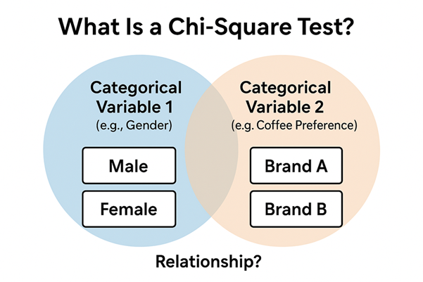
The Chi-Square (χ²) test is defined as a statistical method designed to assess the presence of a significant association between two categorical variables.

Variables in Context

• Variable: A measurable or countable characteristic (e.g., numerical age, recorded preference).
• Categorical Variable: A variable classified into discrete categories or groups. Some of the examples include:
• Gender—e.g., male, female.
• Preferred device type—e.g., iPhone, Android, other.

The Chi-Square test processes categorical data to evaluate whether the distribution of one variable correlates with the distribution of another variable. Examples include determining if phone ownership type correlates with age group, or if test outcomes correlate with study methods applied.

Core Mechanism: Expected Versus Observed

The Chi-Square procedure operates on a single structural comparison: expected frequencies versus observed frequencies.

• Observed Frequencies (O): Numerical values obtained directly from collected data points. Example: from a dataset of 100 instances, 60 instances correspond to coffee preference and 40 instances correspond to tea preference.
  
  
• Expected Frequencies (E): Numerical values projected under the null condition of variable independence. These values are generated using distributional assumptions with no relational influence between variables.

The operational output of the test is a calculated χ² statistic. The magnitude of this statistic represents the squared divergence of observed values from expected values normalized by expected frequencies. A minimal divergence corresponds to random fluctuation, while a substantial divergence indicates the presence of statistically meaningful association.

Types of Chi-Square Tests

Two primary categories of Chi-Square tests exist. Each of these categories serves distinct analytical functions.

1. Chi-Square Test of Independence

This configuration represents the most frequently applied form of the Chi-Square procedure. Its purpose is to evaluate whether a statistically significant association exists between two categorical variables within a single population.

Illustrative Case: A dataset is constructed from a survey measuring two categorical attributes — gender classification and brand preference in coffee selection. The resulting distribution is tabulated for comparative analysis.

• Null Hypothesis (H₀): The categorical variables are independent. No relational structure exists between gender and coffee brand preference.
  
  
• Alternative Hypothesis (Hₐ): The categorical variables are not independent. A relational structure exists between gender and coffee brand preference.
  
  

Execution of the Chi-Square computation produces a χ² statistic. The value of χ² statistic, compared against a critical threshold, provides the decision framework for rejecting or retaining the null hypothesis.

2. Chi-Square Test for Goodness-of-Fit

This configuration is applied to determine whether the frequency distribution of a sample aligns with a predefined or theoretical population distribution. The procedure measures whether the observed categorical frequencies are substantially different from expected frequencies based on earlier data or specified theoretical distribution models.

Example: A distributional claim indicates that a product packaging design leads to consumer choices in specified proportions of—50% red, 30% blue, and 20% green. A dataset of 100 consumer choices is recorded and compared against these proportions.

• Null Hypothesis (H₀): Observed frequencies correspond to the claimed distribution. No significant deviation exists between sample data and theoretical expectations.
  
  
• Alternative Hypothesis (Hₐ): Observed frequencies diverge from the claimed distribution. A significant deviation exists between sample data and theoretical expectations.
  
  

The Goodness-of-Fit test produces a χ² value indicating the degree of alignment or misalignment between observed results and expected proportions. This statistic guides the determination of whether the observed dataset conforms to the hypothesized pattern.

The Chi-Square Formula

The framework of Chi-Square statistic is developed on the comparative examination of observed data values and corresponding expected data values.

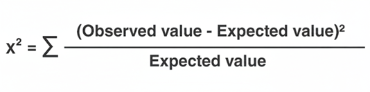
The mathematical expression for the Chi-Square statistic is shown below:

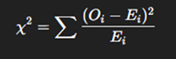
Component Breakdown:

• ∑ (Sigma): Directive to aggregate the computed results across all categorical instances.
  
  
• Oᵢ (Observed Frequency): The actual recorded count for category i in the dataset.
  
  
• Eᵢ (Expected Frequency): The theoretical count for category i, derived under the assumption of independence or predefined distribution.
  
  

The formula operationalizes squared deviations in observed and expected frequencies, normalizes each deviation by the expected frequency, and compiles results into a larger number to yield the final result. 

The larger the χ² value is, the larger the difference between observed and expected frequencies, and greater evidence you have to indicate that two variables are not independent or that the theoretical model does not fit the sample data well.

Step-by-Step Example: Chi-Square Test of Independence

Let's step through a full example with the coffee preference survey. 

Step 1: State the Hypotheses

• Null Hypothesis (H0​): There is no relationship between gender and brand preference for coffee.
• Alternative Hypothesis (Ha​): There is a relationship between gender and brand preference for coffee. 

Step 2: Collect Your Data 

You collected data from 100 individuals. Your results are : 

Observed Frequencies

Step 3: Calculate the Expected Frequencies Now, you need to find out what the numbers should be if there was no relationship.

• Expected Men for Brand A - (Total Men / Total People) x (Total Brand A / Total People) x Total People.
• (50/100) x (40/100) x 100 = 20.
• Expected Men for Brand B - (50/100) x (60/100) x 100 = 30.
• Expected Women for Brand A - (50/100) x (40/100) x 100 = 20.
• Expected Women for Brand B - (50/100) x (60/100) x 100 = 30.

Here is your Expected Frequencies table.

Expected Frequencies

Step 4: Calculate the Chi-Square Statistic Now, use the formula for each cell in the table.

• Cell 1 (Men & Brand A) - 20(30−20)2​=20102​=20100​=5
• Cell 2 (Men & Brand B) - 30(20−30)2​=30(−10)2​=30100​=3.33
• Cell 3 (Women & Brand A) - 20(10−20)2​=20(−10)2​=20100​=5
• Cell 4 (Women & Brand B) - 30(40−30)2​=30102​=30100​=3.33

Now, add them all up to get the final χ2 value. χ2=5+3.33+5+3.33=16.66

Step 5: Interpret the Result A Chi-Square value of 16.66 seems big, but is it big enough? To find out, you compare your calculated value to a critical value from a Chi-Square distribution table. This table uses something called degrees of freedom.

• Degrees of Freedom (df): This is calculated as (number of rows - 1) x (number of columns - 1).
• For our example: (2−1)×(2−1)=1×1=1. So, our df is 1.

Now, using a significance level of 0.05 (which is standard), Chi-Square distribution table would show that for 1 degree of freedom, the critical value is 3.841.

Since our calculated value of (16.66) was very large, we can conclude the difference is statistically significant and we can safely reject the null hypothesis. 

Conclusion

The data indicates that there is a statistically significant relationship between gender and brand of coffee preference. 

Common Misconceptions and Notes

• Correlation and Causation: The Chi-Square test simply tests the indication of the association of one categorical variable to another. It does not determine causal relationships.
• Sample Size: The test requires sufficiently large sample sizes. Expected frequencies below 5 reduce test reliability.
• Data Type: Applicable only to categorical data. Continuous variables are not suitable.
• Expected Frequencies: Expected frequencies represent values under the assumption of independence between variables.
• Magnitude of Difference: The Chi-Square statistic measures deviation between observed and expected frequencies. Larger deviations produce higher Chi-Square values.

Application of the Chi-Square Test

The Chi-Square test is appropriate for assessing associations between categorical variables. Examples include:

• Determining whether a relationship exists between age group and preferred social media platform.
  
  
• Evaluating whether the success rate of a medical treatment varies by patient gender.
  
  
• Investigating the association between political party affiliation and occupation.
  
  
• Assessing whether student performance on a test is influenced by the teaching method applied.
  
  

Computational Considerations

For small datasets it is possible to compute the Chi-Square statistic through manual calculation, but usually we make use of software - R, Python, SPSS, etc. All these tools perform calculations efficiently, thus enabling focus on data acquisition and interpretation.  Online calculators can also be used for rapid verification of results.

Summary

The Chi-Square test helps in the evaluation of how far the observed frequencies depart from the expected frequencies in categorical data. It tells you whether the association you are seeing is statistically significant or simply occurring due to chance. The test is used in various disciplines - including social sciences, medical research, business and marketing - in short it is the primary method for analyzing categorical variables.

FAQs:

Q1. What is the Chi-Square test?

Chi-Square test is a known statistical method with the purpose of evaluating associations between categorical variables.

Q2. When is it used?

It is most often applied in obtaining frequency data to determine whether differences between groups are real or differences due to chance.

Q3. What are the requirements of running a Chi-Square test?

The data must be categorical, the sample sizes must be large enough, at least generally expected cell counts must be greater than 5.

Q4. If the Chi-square value is large, what does this indicate?

The large Chi-Square value provides stronger evidence that variables are not independent, or that the model does not fit the data.